Drop down lists are really useful, especially if you have a table or form that you want other people to complete. By setting rules as to what they can reply will dramatically reduce the time you then spend analysing the answers! In this tutorial I will show you the basics of getting started with drop down lists. Happy learning :)
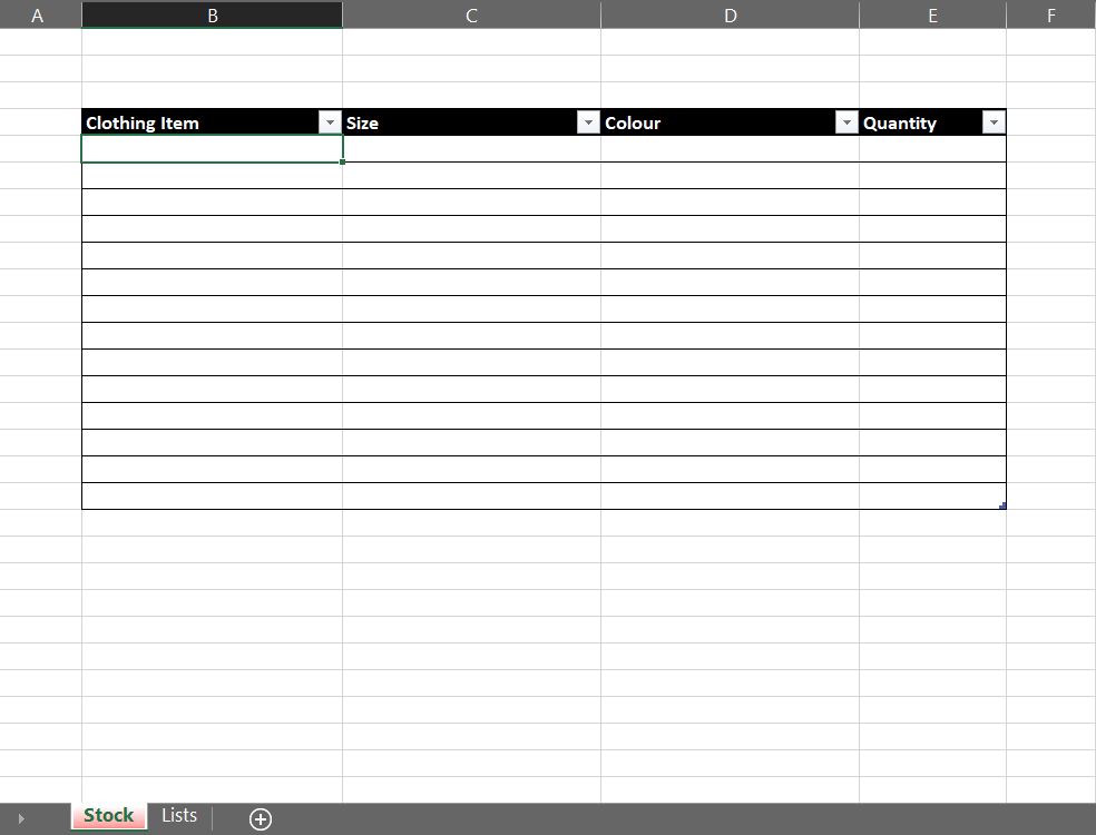
Let’s say for example you are doing a stock inventory and need to complete a table of all the produce currently in stock. Your table will be in one sheet, and in order to create the drop down lists, you will need to create a new sheet for the lists. You’ll see below I have one sheet I’ve called Stock, and a blank sheet that I’ve named Lists…
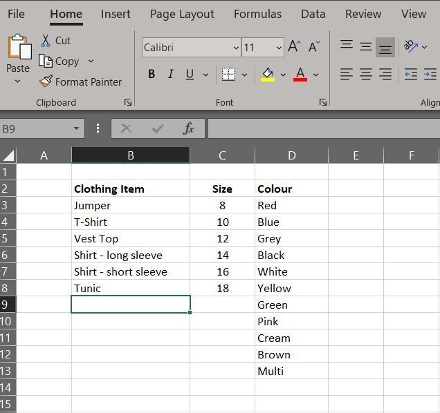
In the lists sheet you need to create lists of the different criteria, so in this example one list will be for the clothing items, another for the sizes, and the final list will be of the different colours…
Step 1
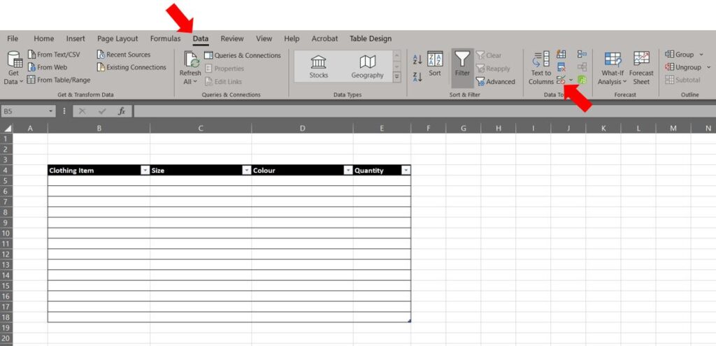
To add the lists as a drop down option in the main table, first select the cell you want the first list to be located, e.g. in our example below it would be the first cell under Clothing Item, cell B5, then go to the Data tab on the ribbon, and click on the icon for Data Validation over in the Data Tools section (if you are unsure which icon it is, hover over them and it will tell you)…
Step 2
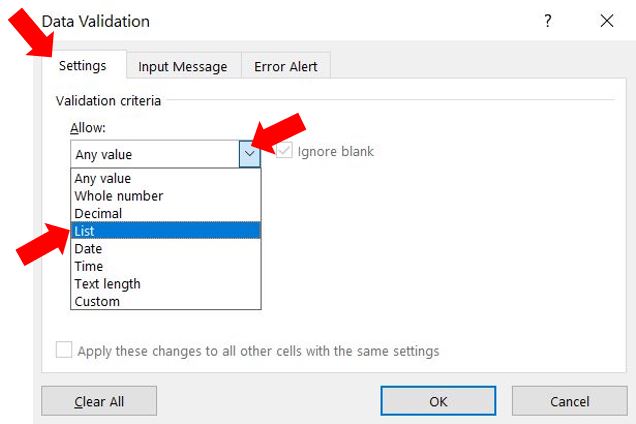
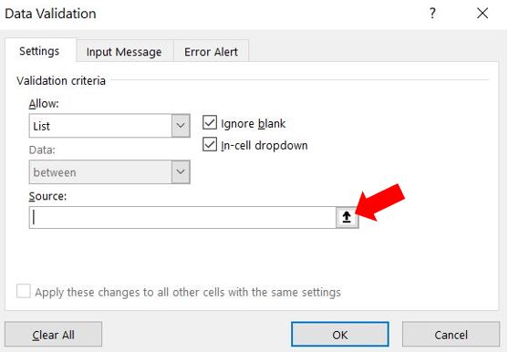
This opens up the Data Validation dialog box. Under Allow, click the drop down arrow and select List…
Step 3
Next you need to tell it where the data is located, so click on the arrow on the right of the Source box…
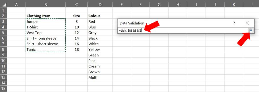
Then click through to the Lists sheet and highlight the data in the Clothing Item list, then click back on the arrow once the range has been entered…
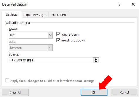
You’re now back in the dialog box where you just click OK and it will take you back to the cell in your table where you’ll now see a drop down arrow. Click on the drop down arrow & you’ll see the list of clothing items you can choose from…
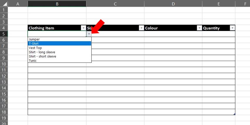
Step 4
To quickly copy the drop down arrow to the rest of the cells in the Clothing Item column, drag the fill handle in the bottom right corner of the cell down the rest of that column in the table. Or you can press Ctrl+C (to copy), highlight the cells in that column and press Ctrl+V (to paste). To check click into one of the other cells and you should see a drop down arrow…
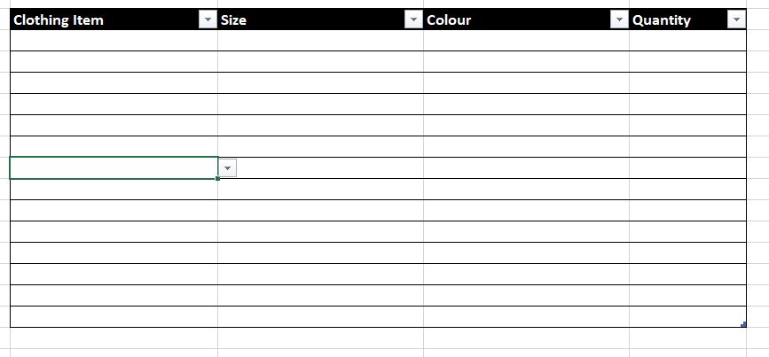
That’s one column complete so you just need to follow Steps 1 – 4 above for the other columns, making sure in Step 3 that you add the range specific to that column from the Lists sheet, then just copy the drop down arrow down the rest of that column…
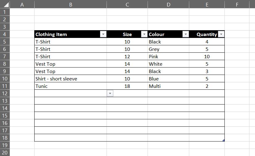
Delete drop down lists
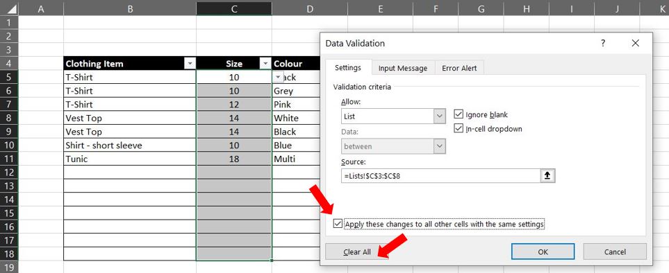
If you want to remove a drop down list, click into the cell you want removing, go to the Data tab on the ribbon, click into Data Validation and click Clear All this will remove the drop down list from only the cell you’re in. If you want to remove the drop down list from the whole column, then tick the box Apply these changes to all other cells with the same settings BEFORE clicking Clear All…
That’s it – a simple step by step way of adding a drop down list to your table in Excel – I hope you found it useful :)
