If you’re new to using Google Sheets, then it might take you a while to get used to where things are located… especially if you’ve been using Excel for a number of years, like I have! Whenever I create a new spreadsheet the chances are I will need to include a date somewhere within it. In this tutorial I show you how to change the date format to one that you prefer. If you want to watch the video showing same then scroll down to the end of this post :)
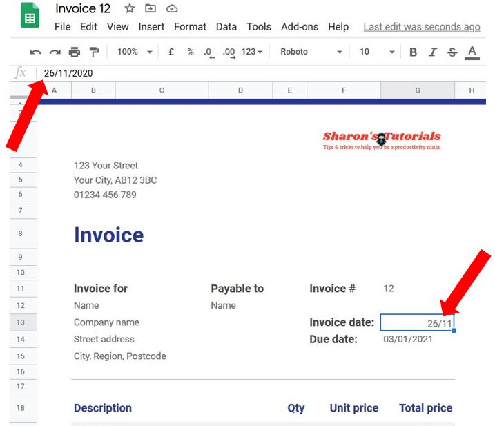
Firstly go into your spreadsheet in Google Sheets where you want the date to be. In the example below, I’m using an invoice that was created from a template (if you want to know how to do that, watch my video here). I want to input a date in cell G13 for the invoice date. If I type in today’s date, you’ll see it has formatted it just as the day and month – even though I have typed out the full date (which you can see in the formula bar at the top)…
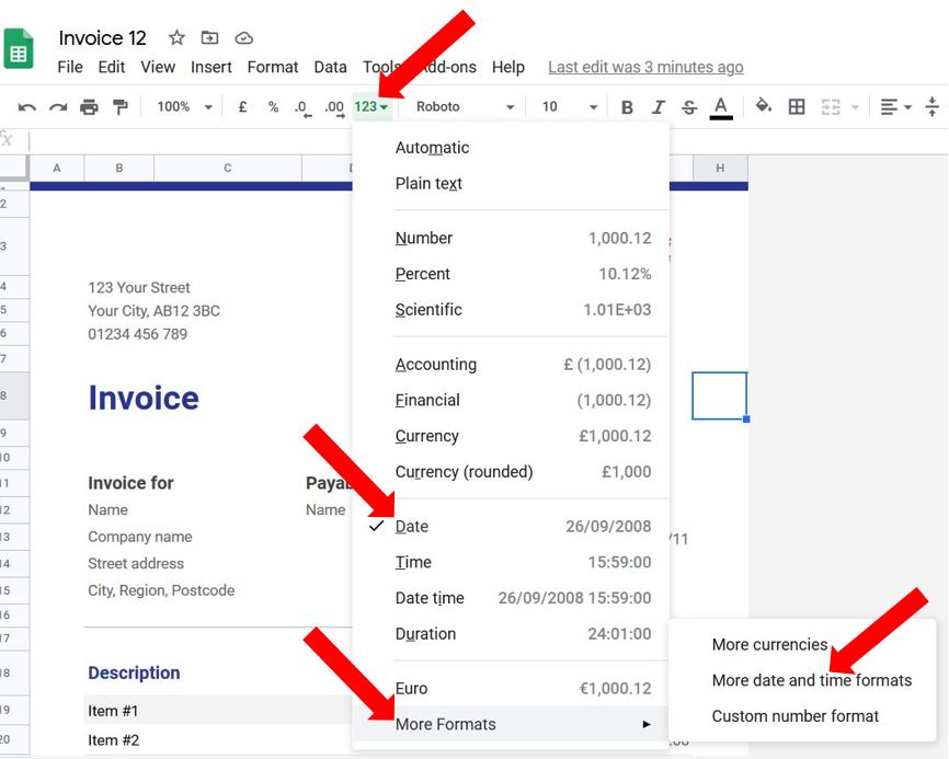
To change the format of the date, click the 123 button in the toolbar at the top of the page, and you’ll see the option of a short date format listed. If you don’t want to use that one, hover over More Formats, and select More date and time formats…
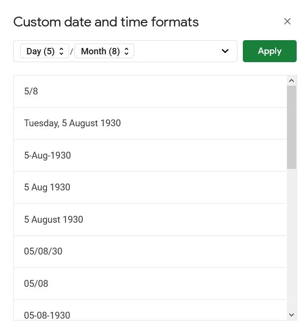
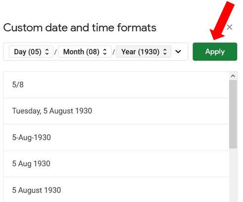
This opens up the Custom date and time format options. You can see my date was showing as 26/11 because only the day and month are currently chosen. Scroll down through the list and choose whichever format you prefer…
Once you’ve selected one, you’ll see it appear in the text box at the top. If you click on the small arrows to the right of each part of the text box, you’ll have even more formatting options and if you want to remove that particular format then just click on Delete…
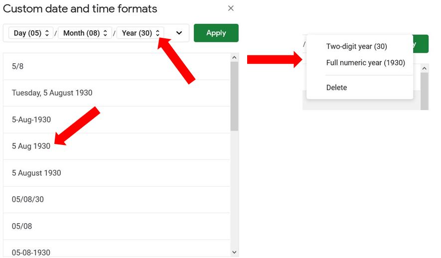
Once you’re happy with the format, click the green Apply button on the right…
And the new date format will be applied. That’s all there is to it! Google Sheets is a big learning curve but once you’re used to where things are positioned, you’ll soon get the hang of it. If you have any questions, let me know in the comments below & I’ll see if I can help :)
