I love working in Google Sheets and use it all the time – here are a few tips I’ve picked up along the way which you need to know if you work in Google Sheets. I’ve also included the video at the end showing all of them – enjoy :)
1. Open new spreadsheet
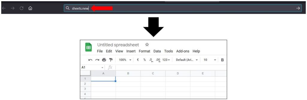
There is a real fast way to open a new sheet – type sheet.new or spreadsheet.new in your browser and it will open up a blank new Google Sheet! How easy is that? You need to be logged into your Google account for this to work first.
This also works for other Google apps as follows:
- To open a new Google doc, type into the browser: doc.new or document.new
- To open a new Google slide, type into the browser: slides.new or presentation.new
- To open a new Google form, type into the browser: form.new
2. Colour rows
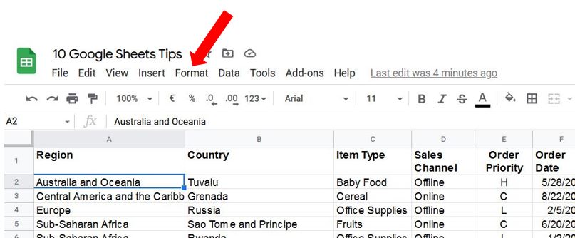
If you have a dataset that is a bit hard to read, you can quickly add colour to it, to make it a bit easier on the eye. Simply click on any cell within the dataset and go to Format in the menu…
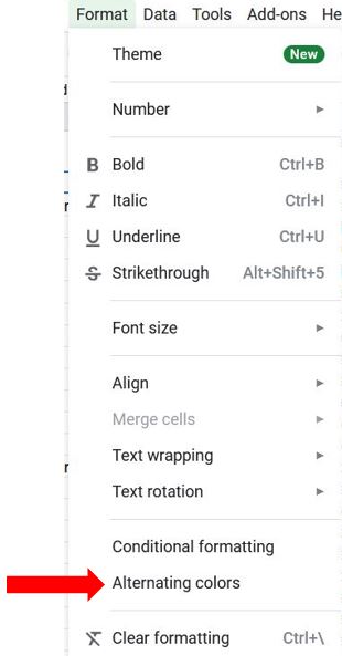
Click on Alternating colors towards the end of the list…
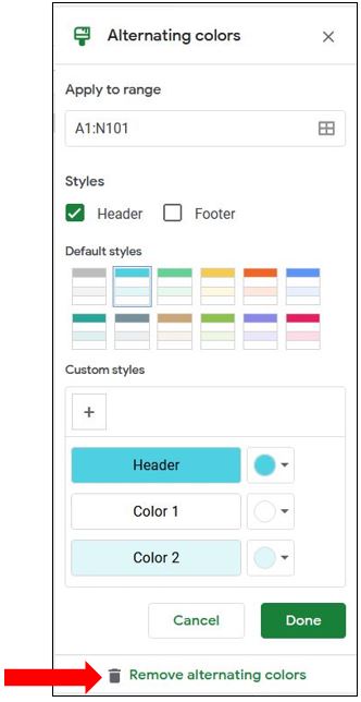
This opens up the alternating colours window where you can select colours from the preset styles, or you can choose your own custom style. You can also tell it whether or not you have a header or footer row in your dataset, and you can select the range that you want it to apply to. Once you’re happy with your selection, click Done…
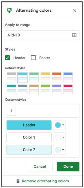
If you want to remove the alternating colours at any time, click on Format, then Alternating colors, and select Remove alternating colors at the bottom of the window…
3. Freeze rows / columns
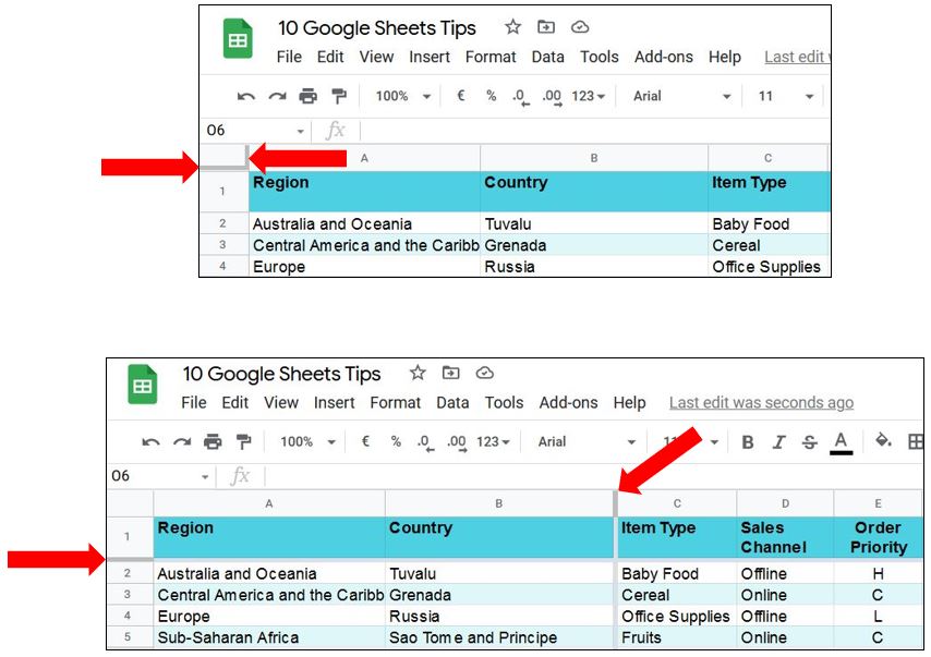
When you have a lot of data set out in tabular form, it’s a good idea to freeze the top row or first column so they remain visible when scrolling down the page. Google sheets has a real quick way to do this! Simply go to the top left corner of the sheet and you’ll see 2 thick grey borders (one on the right of the area and one on the bottom) – hover over these thick lines and the cursor will change to a hand. Click and drag the border line either down (to freeze rows above it), or right (to freeze columns to the left of it). The image below shows I’ve frozen row 1 and across to Column B…
To unfreeze them, just drag the thick grey border lines back to their original position, in the top left corner.
4. Filters
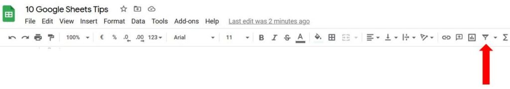
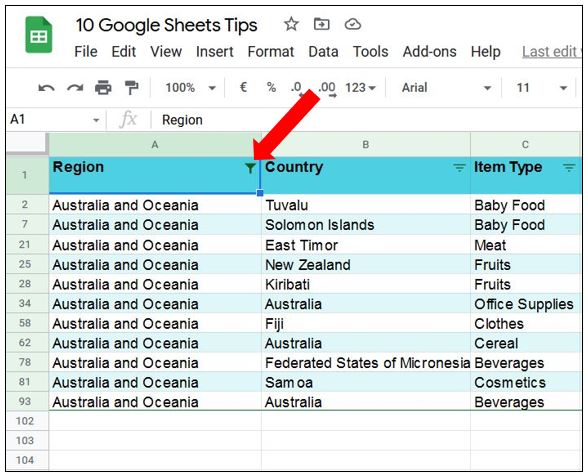
A great way of displaying the information you want to see is to apply filters to your dataset. To turn filters on, first click on any cell within the dataset, then click on the Filter icon (looks like a funnel) over on the right hand side of the toolbar…
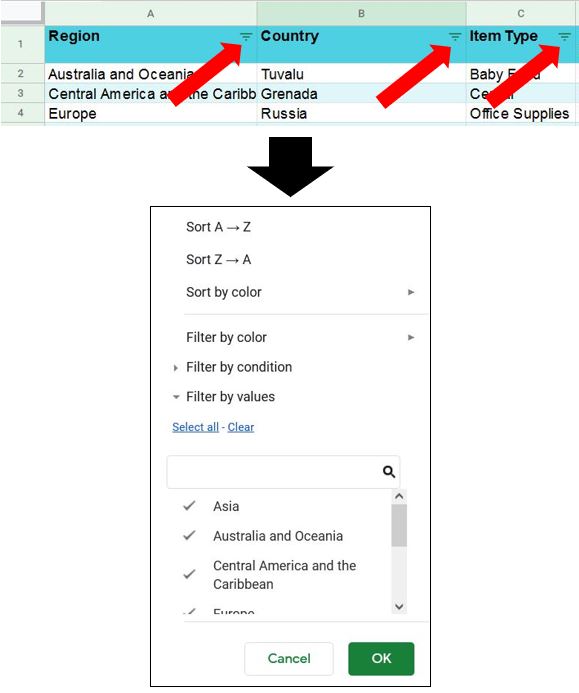
You’ll notice each column header now has a downwards pointing arrow next to the title. Click on the arrow of the column you want to filter and choose the filter option you want, e.g. you can sort the data alphabetically, you can select a certain type from the data e.g. a specific region in the example image below. You can even filter by colour if your cells had certain colours applied to them…
To remove the filters, just click back on the filter icon in the toolbar and it will switch it off.
5. Hide / unhide rows & columns
To quickly hide any row or column, right click on the relevant row or column and select Hide from the options…
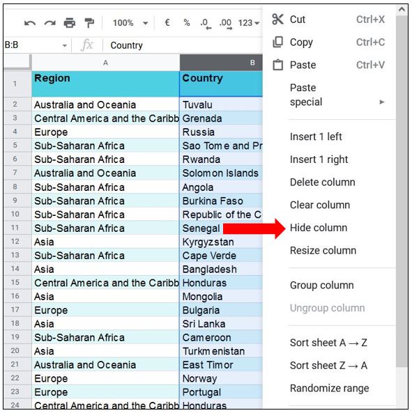
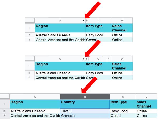
Once it’s hidden you’ll see black arrows in the headers either side of the hidden row or column. Hover over these arrows and a grey box will appear around them, click on one of the arrows and the row(s) or column(s) will unhide…
6. Keyboard shortcuts
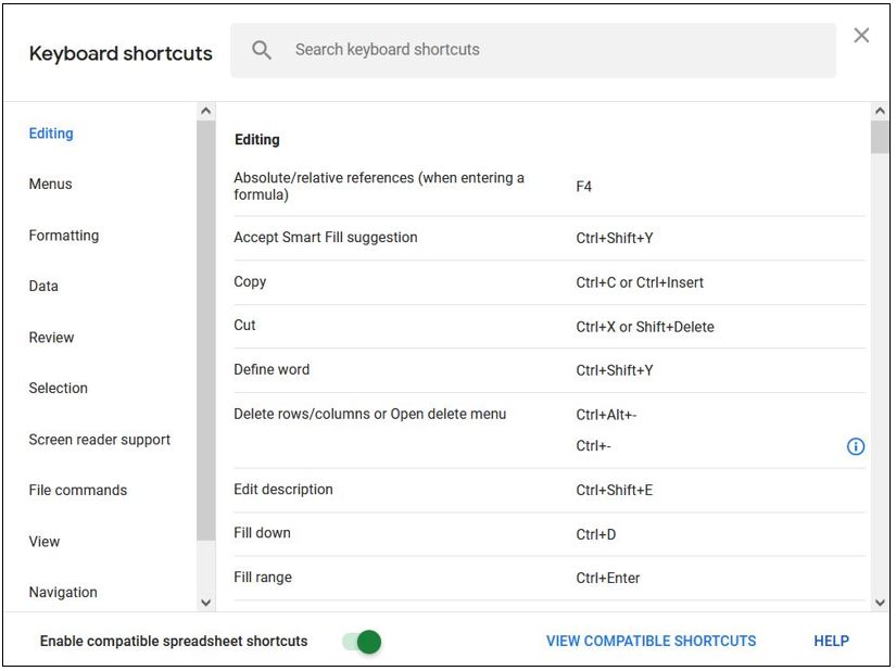
Keyboard shortcuts are a real handy way of saving time when formatting or editing your spreadsheet, but what if you can’t remember them or don’t know if there is a shortcut for what you want to do? Simple, just press Ctrl+/ to open up a list of keyboard shortcuts you can use in Google Sheets – they’re even categorised so you can quickly find what you’re looking for :)
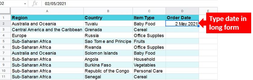
7. Using calendar to enter a date
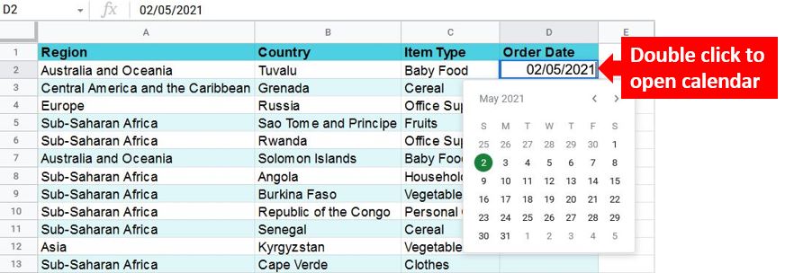
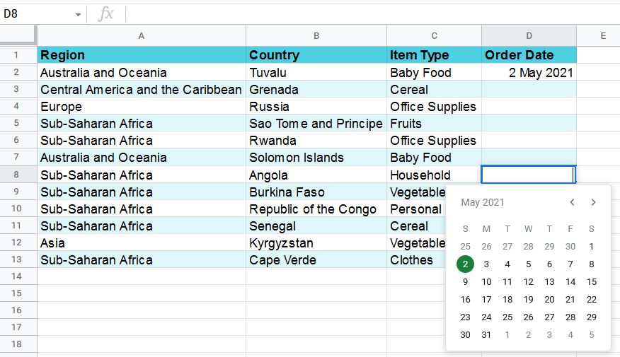
When you enter a date in Google sheets you can actually pick from a calendar, which is really useful! Just type in the date (in long form), click out of it then double click back in it, and it will open the calendar…
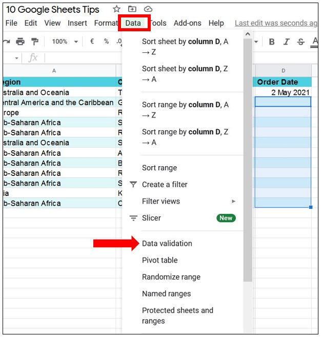
If you want the remaining cells to show a calendar when you click into the blank cell, you can do this through data validation. Highlight the cells you want the calendar to appear in, click on Data in the toolbar then click Data validation…
The range is already selected because you highlighted the cells first, so just click the drop down arrow next to Criteria and choose Date…
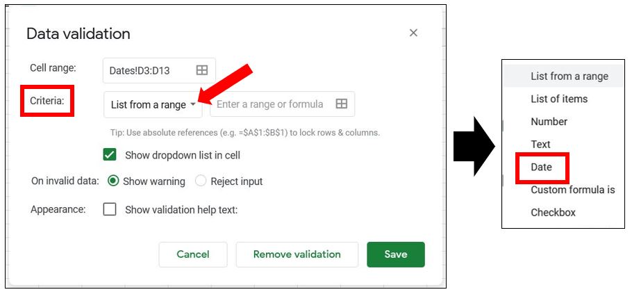
You can also choose whether to reject the input if an invalid date is entered by clicking on Reject input, and you can show some help text if you want to…
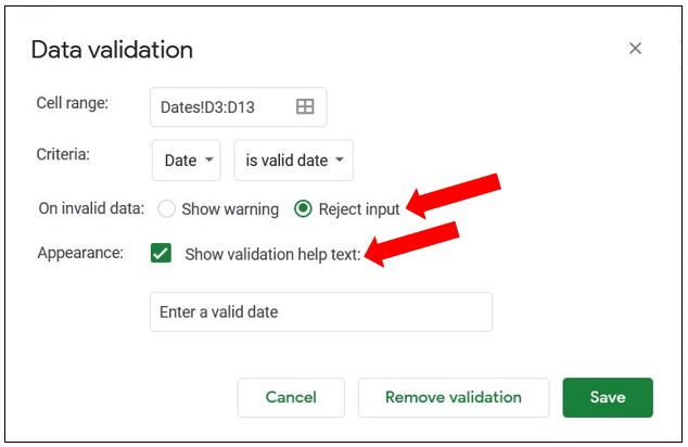
Once you’re happy with the selections, click Save. You can now double click on any of those cells and the calendar will automatically appear for you to choose a date…
If you want to remove the data validation, click on Data, then Data validation and click the button at the bottom called Remove validation.
You may notice that the date formatting is different to the first long form date you entered, if you want all the formatting to be the same read on for the next tip :)
8. Paint format
Using the date example above, you may want all the cells in the Order Date column to be formatted the same as the first entry, i.e. in long date format. There is a real quick way to change the rest – click on the cell you want to copy the format from (in this example it’s cell D2), then click on the paint roller icon over on the left hand side of the toolbar (called Paint format), then highlight the rest of the cells in the column where you want the formatting to apply…
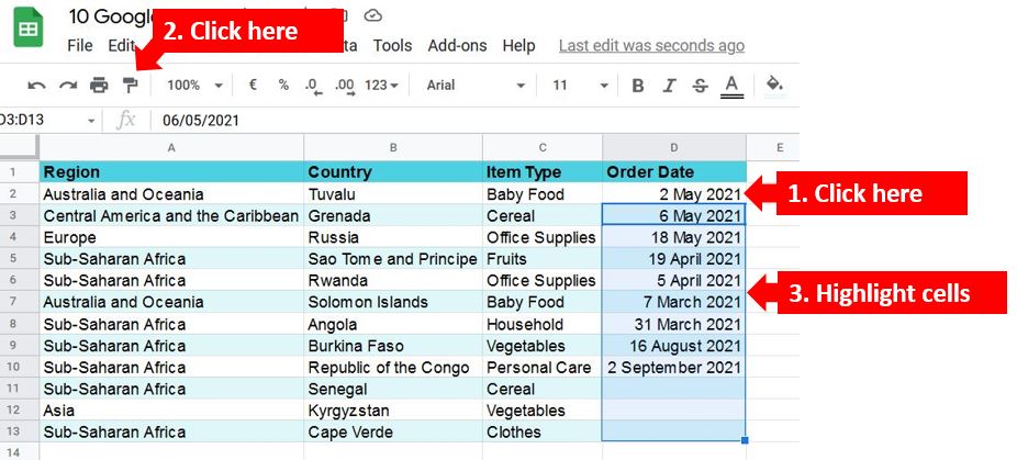
Job done :)
9. Checklist
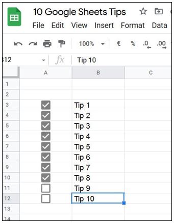
If you want to insert a simple checklist really quickly, first highlight the cells where you want it to go, then click on Insert and select Checkbox towards the end of the list…
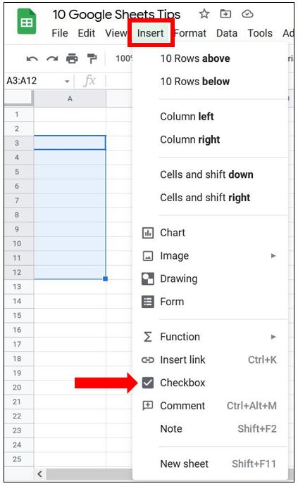
The checkboxes will appear in the cells you highlighted and you can type in a task, or whatever you want to use it for, in the cells adjacent to it. Click on the checkbox to mark it as complete…
10. Download as PDF
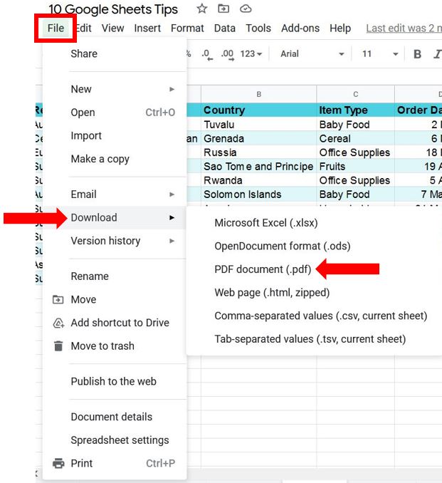
When you want to quickly create a PDF version of your spreadsheet to download, simply click on File, go to Download and choose PDF document…
This will open up the print settings where you can change the orientation of the page, the page size etc. It’s also worth clicking the Formatting and Headers & Footers options over on the right hand side as you can set things like whether to show page numbers, gridlines etc…
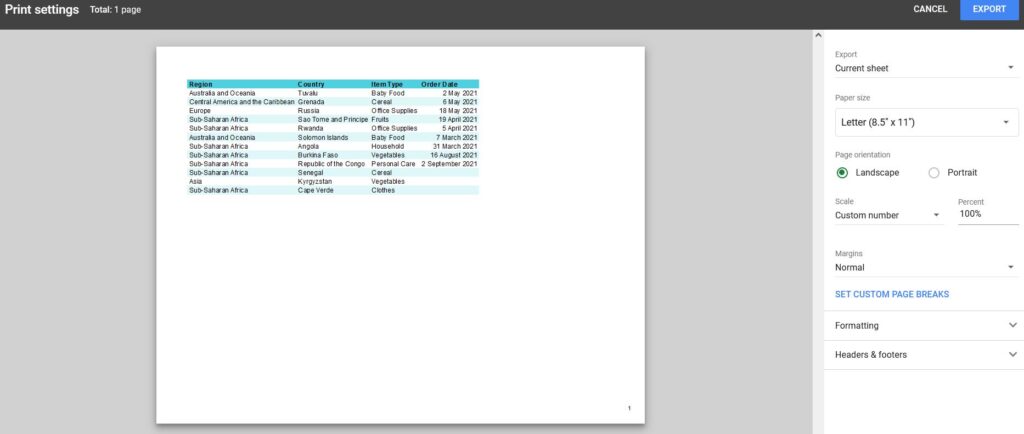
Once you’re happy with everything click on the Export button in the top right corner and it will automatically download it as a PDF file to your PC (in whichever folder your downloads go to).
I hope you’ve found the above tips handy to know – let me know in the comments which is your favourite :)