When you have a sheet full of data, it’s handy to be able to view the column or row headings as you scroll down and across the page. In this tutorial I’ll show you 3 different ways of freezing the view in Google Sheets to make it easier for you :) Check out my video at the end of this post if you prefer to watch this tutorial.
Freeze using your mouse
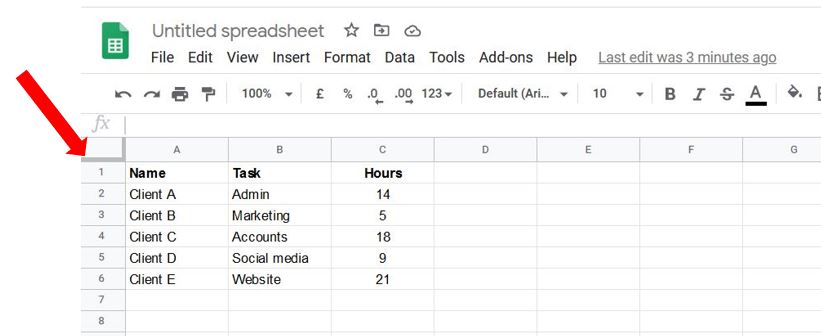
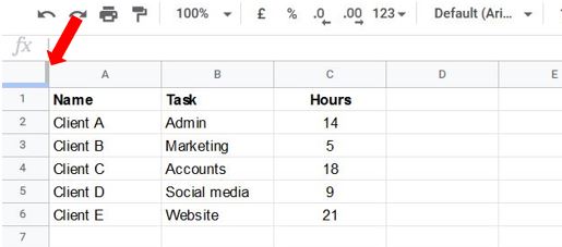
The sheet below is created in Google Sheets and is a basic short list of data. If you look in the top grey square to the left of Column A and above Row 1 you’ll see it has a thicker grey border than the rest…
When you hover over this thick grey border, the cursor changes to a hand symbol…
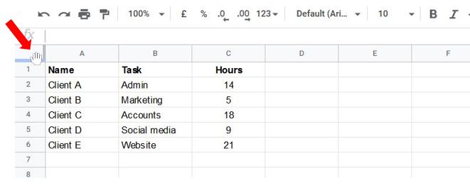
If you left click and hold the mouse when you hover over the bottom thick grey border and drag the border down to the line under row 1, it will freeze the top row…
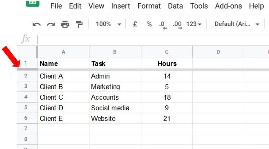
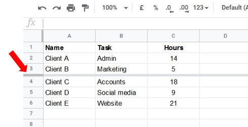
If you want to freeze the top 3 rows, hover over the thicker line so the hand symbol appears, click, hold and drag the line to below row 3…
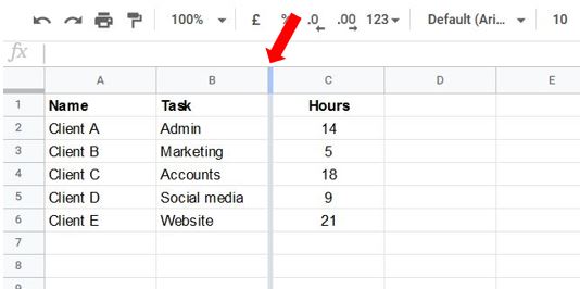
It’s the same process if you want to freeze any of the columns, hover over the thicker border on the right hand side of the grey box…
When the hand symbol appears, left click and hold down your mouse and drag the border to the right stopping after you’ve reached the column header you want to freeze, for example Column B…
If you want to unfreeze any columns or rows, just hover over the grey border, click when it turns to the hand symbol and drag it back to its original position.
Freeze using your keyboard
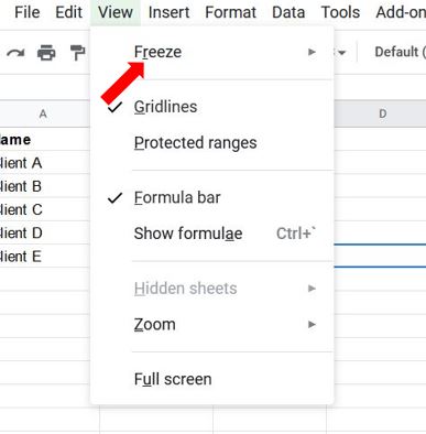
Another way of freezing rows and columns is using your keyboard. If you press Shift+Alt+V this brings up the View menu. You might notice certain letters in the menu are underlined, these are the keyboard shortcuts. So to get to the Freeze options, you would press r (as that’s the letter that’s underlined in the word Freeze on the menu…
This brings up the next set of options for you to choose – if you wanted to freeze the first 2 rows then press w, as that’s the letter underlined in that option…
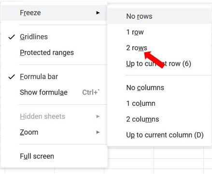
You would do the same for freezing columns, just press the letter for the corresponding options. To unfreeze any rows or columns, type Shift+Alt+V to open the View menu, press r for the Freeze options then press either r for No rows or c for No columns, and they will be unfrozen.
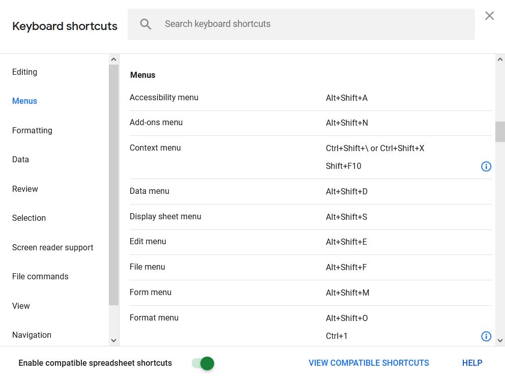
If you want a full list of keyboard shortcuts you can use in Google Sheets, press Ctrl+/ and the full list will appear :)
Freeze using the menu
This last way is using the menu as per above but by clicking on the menu options with the mouse instead of using your keyboard…
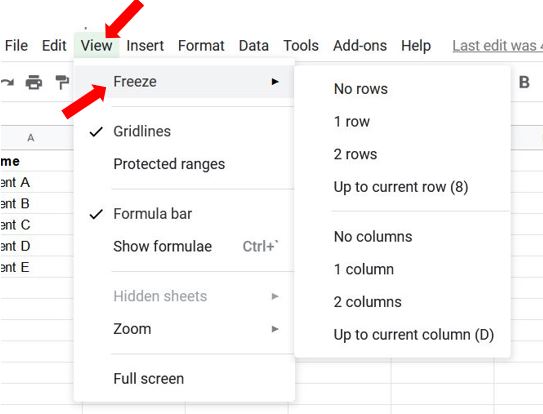
You’ll notice that when you click on View in the menu, there won’t be any letters underlined for shortcut use… this is because they are only activated when you go in using the keyboard shortcut Shift+Alt+V.
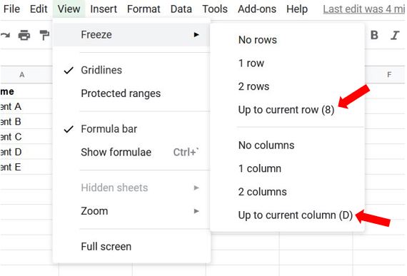
A handy Freeze option in the menu is “Up to current row” which freezes rows above whichever cell is currently selected, and “Up to current column” which freezes columns to the left of whichever cell is currently selected…
So there you have 3 different ways of freezing rows and columns in Google Sheets, I hope you find it helpful :)
