When the ribbon was first introduced in MS Office back in 2007, it was a big learning curve for a lot of users and took people a while to get used to it. Nowadays it feels like it’s always been there and we’d be lost without it :)
There may be times when you feel the ribbon is taking up too much room on your spreadsheet and you just don’t want to see it. This tutorial shows you 5 quick ways to hide (& unhide) it, so only the tab headings are visible. Go to the end of this post if you want to watch the video tutorial instead :)
1. Keyboard shortcut
The quickest way to hide the ribbon is to use the keyboard shortcut Ctrl+F1.
To unhide: press Ctrl+F1 again.
2. Double click
Double click on the active tab heading on the ribbon to minimise it, leaving just the tab headings showing.
To unhide: double click on the active tab heading again.
3. Right click
Right click anywhere on the ribbon and choose Collapse the Ribbon…
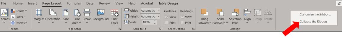
NOTE: This option is called Minimize the Ribbon in Excel 2007 & 2010.
To unhide: Use one of the previous methods above (Ctrl+F1 or double click).
4. Arrow
Look to the bottom right corner of the ribbon and you’ll see an arrow pointing up…
Click on the arrow to minimise the ribbon.
To unhide: Use one of the previous methods above (Ctrl+F1 or double click).
5. Ribbon Display Options
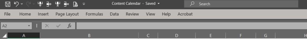
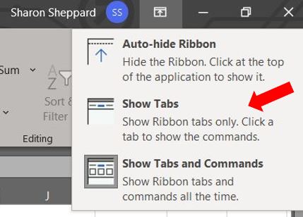
In the top right corner of your screen you’ll see a box with an arrow in it, this is called Ribbon Display Options…
Click this to display the options available to you. To display the tab headings only, click on Show Tabs…
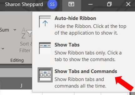
To unhide: Click back on the Ribbon Display Options and select Show Tabs and Commands…
So there you have 5 quick & easy ways of hiding and unhiding the ribbon. I hope you found it useful :)