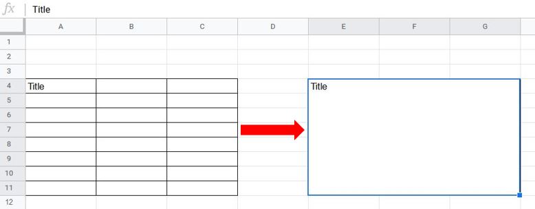
There are times when you want text to be spread over a number of columns or rows – for example you may want the title to span the width of the table. In this step-by-step tutorial I show you how to merge selected cells horizontally, vertically, or both, as well as how to unmerge cells. If you prefer to watch the video, scroll down to the end of this post :)
Whilst merging cells is a great formatting tool to make text look better, it is not recommended to merge cells containing data in a dataset, as it can get a bit messy when it comes to data analysis!
Where to find the Merge cells option
Once you have highlighted the cells you want to merge, there are 2 ways to find the Merge cells option:
Option 1
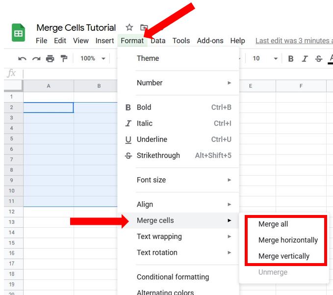
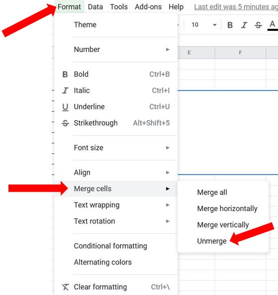
Click on Format in the menu, go down to Merge cells, and select one of the options available to you (depending on the cells highlighted)…
Option 2
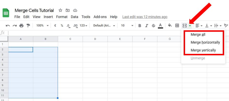
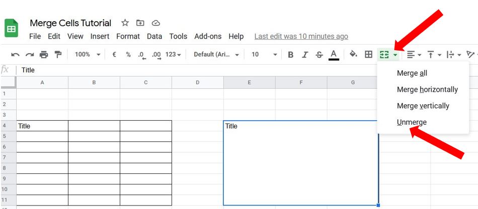
Click on the Merge cells button on the quick access toolbar…
Word of warning!
If you try to merge cells that contain data in more than 1 cell, like the example below…
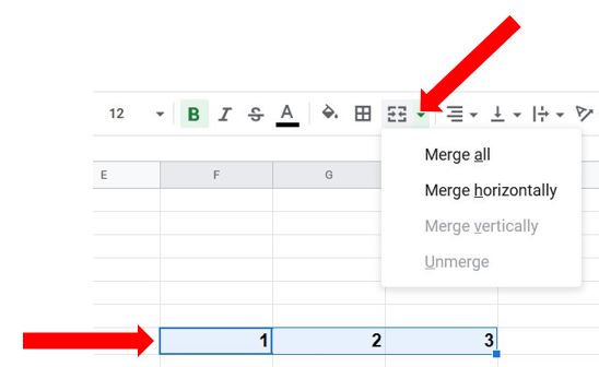
…then you will get the following warning, meaning that only the number 1 will be kept in the example above once the cells are merged…

Below are the 3 different types of merges available in Google sheets:
Merge horizontally
Use this to merge cells across a row (or rows) horizontally…

Merge vertically
Use this to merge cells down a column (or columns) vertically…
Merge all
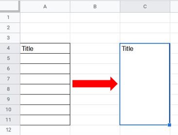
Use this to merge all the cells in your selected range into one single cell…
How to unmerge cells
Select the cells you want to unmerge and either click on Format, Merge cells and then Unmerge…
OR click on the Merge cells button on the quick access toolbar, and select Unmerge…
And that’s how to merge and unmerge cells in Google Sheets – I hope you have found it helpful :)
